Learn with Lin about biophysical characterization: Part I: Light scattering

The ‘Learn with Lin’ series is back!

In this latest article, Lin Wang, alongside Eric Y Hayden, introduces us to biophysical characterization, beginning with light scattering. Exploring how light scattering techniques, particularly dynamic light scattering (DLS) and static light scattering (SLS), help scientists analyze the physical properties of biomolecules such as proteins, Lin and Eric explain the fundamental principles behind Rayleigh and Mie scattering, linking them to everyday phenomena like the blue sky and white clouds. Lin and Eric then delve into DLS, which measures particle size and motion through fluctuations in scattered light, and SLS, which determines molecular weight and interactions. These techniques are essential in formulation development, providing insights into molecular stability and behavior. 

Author’s words:

Hello everyone, this is Lin! It has been more than 3 years since my last article in the ‘Learn with Lin’ series. During my years working in the formulation development field, I have developed a great interest in understanding more about biophysical characterization. In this new series, I invite you to join me as we delve into this captivating realm, exploring the tools that allow us to glimpse into the intricate behavior of proteins in their microscopic universe!

Biophysical characterization is a scientific process used to understand the physical and chemical properties of a protein or other biomolecule. This can include studying its size, shape, structure, stability and interactions with other molecules. Numerous techniques are at our disposal to facilitate this understanding. In this installment, however, we will primarily focus on the fascinating world of light scattering.

So, without further ado, let there be light!

Why is the sky blue and the clouds white?

The colors of the sky and clouds are primarily due to the scattering of sunlight by the atmosphere.

The blue color of the sky is the result of a specific type of scattering called Rayleigh scattering.

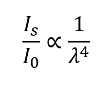
In 1871, Rayleigh attributed the sky’s blue color to sunlight scattering off small particles (smaller than about a tenth of the wavelength of the light) and demonstrated that the intensity of the scattered light is inversely proportional to the fourth power of the wavelength of the light [1]:

Where:

                 I_s is the intensity of the scattered light

                 I₀ is the intensity of the incident light

                λ is the wavelength of the incident light

In the case of the sky, the small particles that scatter the light are primarily nitrogen and oxygen molecules. Blue light has a shorter wavelength and when applying Rayleigh’s scattering formula, it’s evident that shorter wavelengths, such as blue, are scattered more than longer wavelengths, like red.

Figure 1: Diagram of the electromagnetic spectrum

For example, if we consider the average wavelength of red light as 700 nm and blue light as 450 nm, the intensity of blue light scattered is 3.1 times more than red.

This means that as sunlight passes through the atmosphere, the short-wavelength blue and violet light is scattered in various directions across the sky, but the longer-wavelength green, yellow and red light is scattered much less. This is why we see the sky as blue instead of red.

When particles are similar in size to or larger than the wavelength of light, the type of scattering that occurs is called Mie scattering. This is the type of scattering that happens in clouds. Clouds appear white or gray because their water droplets are larger than the wavelength of light, causing them to scatter all colors of light equally; since white light is a combination of all colors in the spectrum, our eyes perceive this uniform scattering as white or gray.

Since Rayleigh scattering is applicable to particles that are much smaller than the wavelength of light, or visible light, this typically means particles that are less than about 1 micrometer in diameter. Many biomolecules, such as proteins, nucleic acids and small cellular components, fall into this size range, making Rayleigh scattering a useful tool for their characterization. Two techniques that effectively utilize this principle are dynamic light scattering (DLS) and static light scattering (SLS).

Dynamic light scattering

DLS is termed ‘dynamic’ because it measures fluctuations in scattered light intensity over time. These fluctuations are caused by the Brownian motion of particles suspended in a fluid medium. The recorded intensity fluctuations are analyzed using a mathematical technique called autocorrelation analysis. Autocorrelation calculates how the intensity of the scattered light correlates with itself at different time intervals. As time progresses, the correlation between intensity fluctuations at different time intervals decreases. Larger particles experience greater resistance in the medium and require more energy to achieve the same motion as smaller particles, resulting in slower movement. This leads to slower fluctuations of light and a more similar correlation with past states. Conversely, smaller particles demonstrate faster fluctuations and faster decay rates. This process can be likened to comparing a ‘snapshot’ of a busy street scene to a snapshot taken slightly later—where the degree of similarity between the two snapshots reflects how quickly the people and cars on the street were moving. The faster the movement, the greater the difference between the two snapshots will be, just as a faster decay in the autocorrelation function indicates smaller particles rapidly changing positions due to Brownian motion. From the decay rates, we can get the translational diffusion coefficient (D_t).

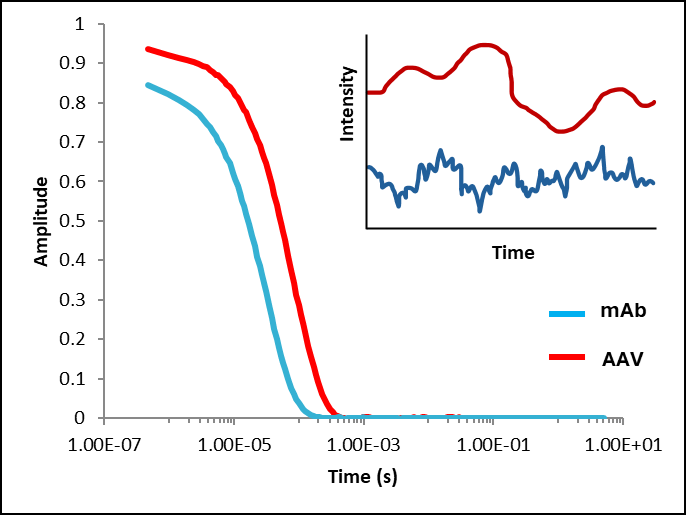
Figure 2: Examples of autocorrelation functions for molecules of two different sizes: blue (monoclonal antibody (mAb), 10 nm) and red (adeno-associated virus (AAV), 27 nm).

MAb shows faster decay in autocorrelation (shifted to the left) compared to the AAV, which shows a slower decay in autocorrelation, (shifted to the right). The graph in the upper right corner is a schematic representation for the DLS intensity fluctuations of mAb and AAV molecules. It illustrates that smaller particles (dark blue) exhibit faster fluctuations in scattered light, whereas larger particles (dark red) display slower fluctuations.

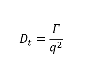
To calculate D_t, we need to get two numbers, the decay rate (Г) and the magnitude of the scattering vector (q).

(1)

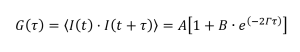
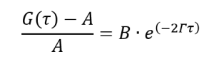
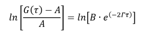
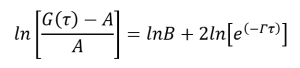
The decay rate can be obtained from the autocorrelation function (G(τ)) by fitting the data to the model as below:

 (2)

Where:

A describes the baseline correlation value at time infinity

B describes the initial correlation value

t is the initial time

τ is the delay time

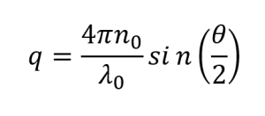
The magnitude of the scattering vector can be obtained from the following equation:

(3)

 

Where:

n₀ is the refractive index of the liquid

λ₀  is the wavelength of the incident light

θ is the scattering angle

Longer wavelengths (e.g., 600–700 nm) are often chosen for DLS because they work well across a broader range of particle sizes, providing a balance between effective scattering and the ability to capture the broader range of particle sizes in typical DLS measurements. For example, the Uncle instrument from Unchained Labs (CA, USA) uses a wavelength of 660 nm [2]. The scattering angle is typically set at 90 degrees (side scattering) but other angles, such as 175 degrees (back scattering), may also be employed in some instruments for various purposes [3].

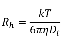
The hydrodynamic radius (R_h) can then be obtained by using the Stokes-Einstein equation.

(4)

Where:

k is Boltzmann’s constant

T is the temperature in K

η is the solvent viscosity

D_t is the translational diffusion coefficient

Cumulants approach, Z-average diameter and polydispersity index [4–7]

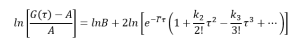
In most practical cases, sample solutions exhibit polydispersity, meaning that the autocorrelation function, G(τ), is a sum of multiple single-exponential decay functions, each corresponding to different decay rates. This complexity makes the fitting process challenging. There are a few methods developed to address this difficulty. For example, for mono-modal distribution, linear fit and cumulant expansion are used, while for non-monomodal distribution, meaning samples with multiple particle sizes, CONTIN (constrained regularization method) and non-negative least squares (NNLS) are used. Among all these methods, cumulants approach is the most common method and will be discussed in detail below.

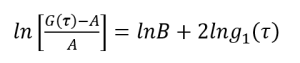
First, let’s make some rearrangements to equation (2):

(5)

(6)

(7)

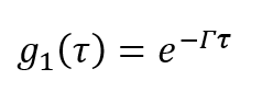
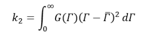
Now let’s define a function g₁(τ),

(8)

(9)

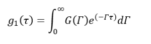
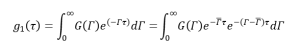
For a polydisperse system, g₁(τ) cannot be expressed as a single exponential decay anymore but an intensity-weighted integral over a distribution of decay rates G(Г).

(10)

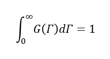(11)

Next, we will define an average decay rate (  and make a rearrangement of g₁(τ),

(12)

To account for polydispersity,

(13)

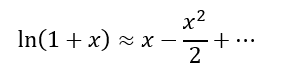
We will use a power series expansion here,

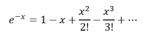(14)

Expand  in equation (13),

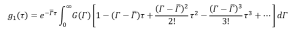(15)

Where,

Now,

(16)

Where,

Now let’s go back to equation (9) and substitute g₁(τ) with equation (16),

(17)

We know that,

And x² << x, can be negligible,

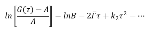(18)

 

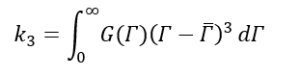
Take equation (1), (3) and (4), we can get the Z-average,

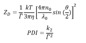
The Z-average diameter is the intensity-weighted mean hydrodynamic size of a collection of particles. PDI is used to indicate the width of the distribution. PDI less than 0.1 indicates a highly uniform particle size; PDI greater than 0.7 commonly indicates a very broad range of particle sizes. The calculations for these parameters are defined in the ISO standard document ISO 22412:2017.

Diffusion interaction parameter

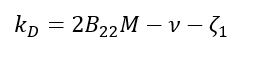
Another powerful application of DLS is the assessment of reversible, nonspecific interactions by determining the diffusion interaction parameter (k_D).

In an ideal dilute solution, the diffusion coefficient (D_t) is not dependent on solute concentration. However, when concentration increases, the solution becomes less ideal. If the concentration is not very much higher than dilute, the measured diffusion coefficient may be expanded in a power series as [8]:

At low concentrations, the higher-order terms contribute very little to the overall value of D_t. Therefore, the first-order term is usually sufficient to describe the concentration dependence of the diffusion coefficient. Attractive interactions (k_D < 0) cause an apparent decrease in the diffusion coefficient. Repulsive interactions (k_D > 0) cause an apparent increase in the diffusion coefficient.

To determine k_D, follow these steps:

1. Prepare a series of samples with a range of concentrations (typically lower than 10 mg/mL) of the molecules of interest.
2. Use DLS to measure the D_t for each concentration.
3. Plot the measured D_t against the corresponding concentrations (c).
4. Perform a linear regression on the plotted data. The value of k_D will be determined using the slope of the line obtained from this fit, divided by the intercept (D₀). The graphical representation of this is called the Debye plot.

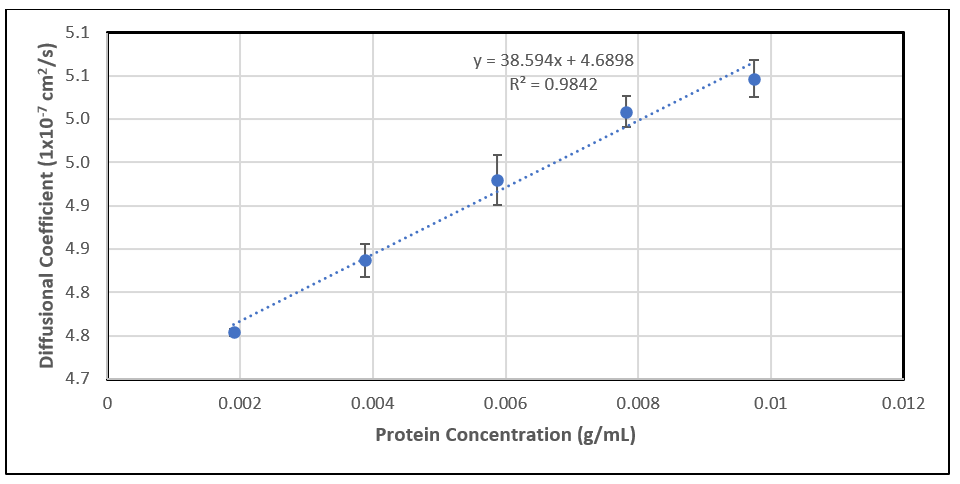
Figure 3: A typical regression plot for k_D determination.

Static light scattering, the average molecular weight and the second virial coefficient

Unlike DLS, SLS makes use of the time averaged intensity of scattered light, without considering the time-dependent fluctuations in the scattered light intensity. SLS is a valuable tool for determining the average molecular weight, and other key properties of macromolecules and nanoparticles.

In this section, we will explain how SLS can be used to obtain two crucial parameters: the average molecular weight (M_W) and the second virial coefficient (B₂₂ or A₂).

We will start with the Rayleigh equation [9]:

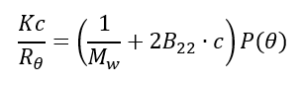
Where:

R_θ is the ratio of scattered light to incident light of the sample. The standard approach to obtain R_θ involves measuring the scattering intensity of the sample relative to that of a common standard, toluene.

I_A: Residual scattering intensity of the analyte; I_T: Toluene scattering intensity; n₀: Solvent refractive index; n_T: Toluene refractive index; R_T: Rayleigh ratio of toluene.

M_W is the average molecular weight

B₂₂ is 2nd virial coefficient

C is concentration

P (θ) is the form factor describing the angular dependence of the sample scattering intensity

K is the optical constant as defined below:

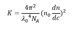
Where:

N_A is the Avogadro’s constant

λ₀ is the laser wavelength

n₀ is the solvent refractive index

dn/dc is the differential refractive index increment, a measure of how much the refractive index of a solution changes with respect to a change in the concentration of its solute and is available in the literature for many sample/solvent combinations

When the particles in solution are much smaller than the wavelength of the incident light (<λ₀/20), multiple photon scattering will be avoided. Under these conditions, P(θ) will reduce to 1 and the angular dependence of the scattering intensity is lost. The Rayleigh equation will be simplified to:

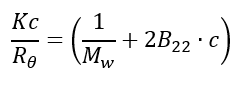
If we plot Kc/R_θ against concentration c and perform a linear regression on the plotted data, the intercept will be 1/Mw, and B₂₂ can be obtained from the slope.

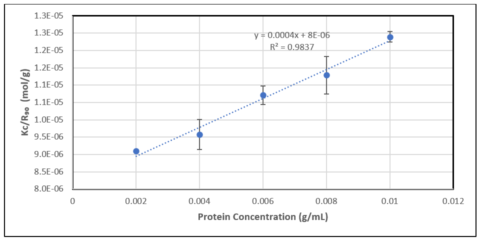
Figure 4: A typical regression plot for B₂₂ determination.

When a solution is not ideal, to account for intermolecular interactions, the osmotic pressure can be expressed using a virial expansion [10]:

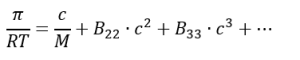
At low concentrations, higher-order terms (such as B₃₃, c³, etc.) become negligible.

The second virial coefficient B₂₂ specifically accounts for pairwise interactions between pairs of identical solute molecules. A positive B₂₂ signifies that the primary interaction between molecules is repulsive. A negative B₂₂ indicates attractive interactions.

Please note that there is some debate regarding whether the measurements made via light scattering actually represent A₂ values, as opposed to the B₂₂ values traditionally obtained by analytical ultracentrifugation. The B₂₂ value derived from light scattering is influenced by a combination of protein-protein and protein-buffer interactions, particularly in formulations with high salt concentrations [11].

The relationship between B₂₂ and k_D

The equation relating B₂₂ and k_D is typically expressed as [12]:

Where:

M is the molecular weight

v is the partial specific volume

ζ₁ is a first-order concentration coefficient of friction, representing the interaction between solute molecules and the solvent.

The hydrodynamic term (ζ₁ + v) is often proportional to B₂₂, so empirical relationships are usually reported as below, where a and b are constants:

Both B₂₂ and k_D can describe the non-ideality of the solution. It should be mentioned that large positive k_D usually indicates strong repulsive interactions, or positive B₂₂. However, a negative k_D does not necessarily mean that B₂₂ is negative.

Kirkwood-Buff integral (G₂₂)

Here, we will also briefly touch on G₂₂, the protein–protein Kirkwood–Buff integral. While B₂₂ and k_D typically work for low protein concentrations (< 20 mg/ml), G₂₂ accounts for protein crowding effects that give rise to strongly attractive or repulsive interactions and is more appropriate for solutions with high concentrations, where short-range intermolecular interactions become more prominent [13].

G₂₂ is linked to the Rayleigh ratio by the following equation:

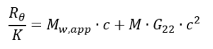
Where:

M is the theoretical molecular weight

M_{W, app} is the apparent molecular weight

c is the protein concentration

M_{W, app} equals M when in ideal solutions, but differs when there are strong protein–solvent and protein–cosolute interactions.  M_{W, app} and G₂₂ can be obtained by regressing the data R_θ/K with concentration using non-linear fitting [14].

Unlike B₂₂ and k_D, G₂₂ indicates the opposite: positive values for attractive interactions and negative values for repulsive interactions.

Summary

In this article, we have explored the fundamentals of DLS and SLS, including key parameters such as Z-average, PDI, k_D, B₂₂, G₂₂ and average molecular weight. While both techniques are valuable for understanding the behavior and stability of colloidal systems, DLS is more often used to measure the size and size distribution of molecules in a solution, and SLS can be used to determine the average molecular weight and quantify molecular interactions as B₂₂ and G₂₂ via the concentration dependence of the scattered intensity. Notably, a widely used application of SLS for molecular weight determination is multi-angle light scattering (MALS), especially when coupled with other instruments, such as in SEC-MALS. This topic, along with other biophysical characterization techniques like AUC, may be addressed in future installments. Stay tuned!

---

You may also be interested in:

• Learn with Lin about therapeutic antibodies: part I − an introduction
• Learn with Lin about therapeutic antibodies: part II − how it works
• Learn with Lin: part I – basic terms in LC–MS
• Learn with Lin about LC–MS bioanalysis: part II – get to know the system
• Learn with Lin about LC–MS bioanalysis: part III tune the triple quadrupole system
• What is toxicology?
• What is chromatography and how does it work?

---

Meet the authors

Lin Wang
Scientist
Regeneron Pharmaceuticals (NY, USA)

Lin Wang is a Scientist in the Formulation Development group at Regeneron Pharmaceuticals, where she leads developability assessments for biologic candidates across various indications, including anti-SARS-CoV-2 and immuno-oncology. With over 10 years of industry experience, Lin specializes in formulation development, analytical method development and stability assessments of therapeutic monoclonal antibodies. She holds a Master of Science in Chemical Engineering from Rutgers University (NJ, USA) and a Bachelor of Science in Chemistry from Xiamen University (China). Lin is passionate about driving CMC strategies, supporting IND/BLA filings and fostering collaboration across drug development phases.

Eric Y Hayden
Principal Scientist
Regeneron Pharmaceuticals (NY, USA)

Dr Eric Y Hayden is a Principal Scientist at Regeneron Pharmaceuticals, Inc. in the Protein Development group within the Therapeutic Proteins Department. He works closely with the Neuroscience therapeutic focus area to study and develop therapeutics for neurodegenerative diseases. He was previously Assistant Project Scientist and Postdoctoral Scholar in the Department of Neurology in the David Geffen School of Medicine at the University of California, Los Angeles (USA). He has a long held curiosity in protein folding and misfolding as it relates to neurodegenerative diseases. His research has examined the biophysical and biochemical properties of amyloid forming proteins, and their oligomeric assemblies. Dr Hayden’s doctoral work at Albert Einstein College of Medicine (NY, USA) focused on studies of the molecular basis of Parkinson’s disease, examining α-synuclein oligomerization, fibrillation and inhibition. In his postdoctoral work he developed a technique to stabilize large quantities of amyloid β-protein (Aβ) oligomers, and developed methods to isolate individual oligomers. His work identified critical regions of the Aβ sequence through D-amino acid scanning substitutions. In collaboration with clinicians, he led biomarker development studies examining the ability of cerebrospinal fluid to inhibit oligomerization, and investigated mixed dementia in a novel mouse model to understand the interplay between stroke and Alzheimer’s disease.

Dr Hayden received a Bachelor of Arts in Biology from New York University (USA), and an MS and PhD in Physiology and Biophysics from Albert Einstein College of Medicine. He performed postdoctoral research with David B Teplow in the Department of Neurology at UCLA, and worked with Jason Hinman also in the UCLA Department of Neurology. He has been recognized for his research through awards including pre-doctoral and post-doctoral training grants from the NIH, the Outstanding Young Alumni Award from The Albany Academies, the 2012 Mazz Prize from the UCLA Department of Neurology, a Rapid Grant Award from the UCLA Claude Pepper Older Americans Independence Center and the UCLA Clinical and Translational Science Institute, the 2013 Young Investigator Award from the California Southland Chapter of the Alzheimer’s Association, and the 2017 Turken Research Award from the Easton Center for Alzheimer’s Disease Research at UCLA.

---

Disclaimer: the opinions expressed are solely those of the authors and do not express the views or opinions of Bioanalysis Zone or Taylor & Francis Group.